Reading: Treating Inflation Consistently

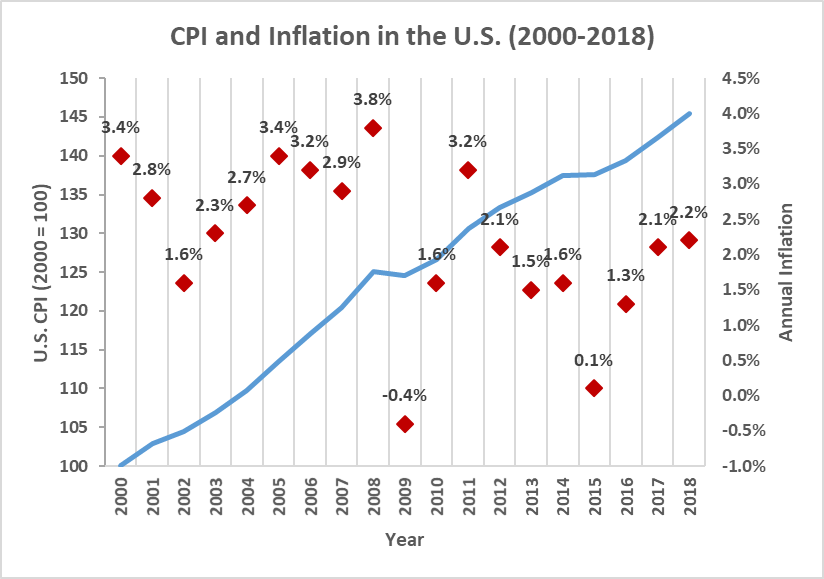
The following figure summarizes the development of U.S. consumer prices over the period 2000-2018. The data are from the Federal Reserve Bank of Minneapolis:

• The blue line shows how the price of a standard basket of consumer goods has evolved over time. This is the so-called Consumer Price Index (CPI). We have indexed the price to 100 in the year 2000.
  
  
• The CPI increases from 100 in the year 2000 to 145 in the year 2018. The interpretation of this development is straightforward: The same basket of goods that cost $100 in 2000 cost $145 in 2018.
   
• Consequently, the consumer price level has increased by 45% over the 18 years under investigation. This corresponds to an average annual increase of 2.1%.
   
• The red dots in the graph show the annual rate of inflation. It is the percentage change in the CPI from one year to the next. In 2000, for example, the annual inflation was 3.4% whereas in 2018, it was 2.2%. As we have just learned, the average annual rate of inflation was 2.1% between 2000 and 2018.
   

Discussion

• Because of inflation, the purchasing power of money falls over time. According to the numbers above, an employee who earned $60'000 in 2000 could buy 600 baskets of consumer goods at a price of 100 in 2000:
   
  \( \frac{Salary_{2000}}{CPI_{2000}}=\frac{60'000}{100}=600\).
   
  the same salary only bought 414 baskets of these baskets in 2018:
   
  \(\frac{Salary_{2018}}{CPI_{2018}}=\frac{60'000}{145}=414\).
   
• Consequently, whereas the salary remained constant in nominal terms (actual dollars), it dropped considerably in real terms (once we take inflation into consideration).
   
• To express the employee's salary in real terms, we can factor out the loss in purchasing power due to inflation by dividing the end-of-period salary by one plus the cumulative inflation. In the example above, with a cumulative inflation of 45%, a salary of $60'000 in 2018 buys the same amount of goods as a salary of 41'379 in 2000. Let's use the Greek letter pi (\(\pi\)) to denote the rate of inflation:
    
  \( \text{Real salary 2018 (in 2000 dollars)} = \frac{\text{Nominal salary 2018}}{1+\pi} \) \( =\frac{60'000}{1.45} = 41'379 \) 
   
• The process of expressing future cash flows in past purchasing power is called deflating. The resulting cash flow is the real cash flow (expressed in 2000 dollars)
   
• Many managers and decision makers find it more practical to work with deflated (real) cash flows, as deflated cash flows are more easily comparable over time. To find the deflated value of a future cash flow, we simply divide that future cash flow by one plus the expected inflation.

Example

A manager currently earns $120'000. He expects his salary to increase to $150'000 over the next 3 years. Expected inflation over that period is 10%. Based on this information, by how much will the manager's real salary increase?
 

To find the answer, we can deflate the expected salary in 3 years ($150'000) by dividing it by one plus the expected inflation (\(\pi\)) of 10%:
  

\( \text{Real salary 3 (in today's dollars)} = \frac{\text{Nominal salary 3}}{1+\pi} \) \( =\frac{150'000}{1.10} = 136'364 \) 

Expressed in today's dollars, a salary of $150'000 in 3 years is equivalent to a salary of $136'364 today in terms of purchasing power. Consequently, in real terms, the manager's salary is expected to increase by 13.6%.

Nominal and Real Rates of Return

The same considerations apply to asset returns. Expected returns should compensate investors for two dimensions:

• The loss in purchasing power the investor suffers during the investment period due to inflation.
• The real return the investor requires to forego consumption today and accept the risk of the asset.

Let's consider an investor who requires a real return of 10% on an investment of $100 that lasts 1 year. Put differently, in order to part with her money and accept the risk of the asset, she wants to be able to consume 10% more in one year. Expressed in today's dollars, she therefore wants a repayment of 110 in one year.

Now let's assume the expected rate of inflation (\(\pi\)) is 5%. If so, we know from the considerations above that a payment of $115.5 in one year will have the same purchasing power as $110 today:  
 

\(\text{Nominal repayment}_1 = \text{Real repayment}_1 \times (1+\pi) \) \(=110 \times 1.05 = 115.5 \)

The total nominal rate of return (R), therefore is 15.5%.  This nominal return consists of two elements: A real rate of return (R* = 10%) and a compensation for inflation (π =5%). The relation between the three dimensions is the following:
  

\( R = (1+R^*) \times (1+\pi) - 1 = 1.1 \times 1.05 - 1 = 0.155 = 15.5\% \)

Similarly, we can find an asset's real rate of return (R*) by solving the above expression for R*:
 

\(R^* = \frac{1+R}{1+\pi} -1 \)

Therefore, as in the case of cash flows, we can find the real rate of return by deflating the nominal rate of return with the expected rate of inflation!

Example

An investment promises a nominal rate of return (R) of 25%. The expected cumulative inflation (\(\pi\)) over the investment period is 12%. Based on this information, what's the investment's real rate of return (R*)?

Using the equation above, we find a real rate of return of 11.6%:

\(R^* = \frac{1+R}{1+\pi} -1 = \frac{1.25}{1.12}-1=0.116 = 11.6\%\)