Reading: WACC for Listed Firms
So far, we have seen what the WACC is and how we use it in firm valuation. This section takes a brief look at how to estimate the WACC in practice.
2. Estimating the Cost of Equity
2.4. Estimating Beta
We are left with the computation of beta. One solution is to estimate a regression of the form:
\( r_{jt} = \alpha_j + \beta_j \times r_{Mt} + \epsilon_{jt} \).
where:
\( r_{jt} \) = continuously compounded stock return of firm j measured from month (t-1) to month t;
\( r_{Mt} \)= continuously compounded market return measured from month (t-1) to month t;
\( \epsilon_{jt} \) = error term;
\( \alpha_j \) , \( \beta_j \) = regression coefficients.
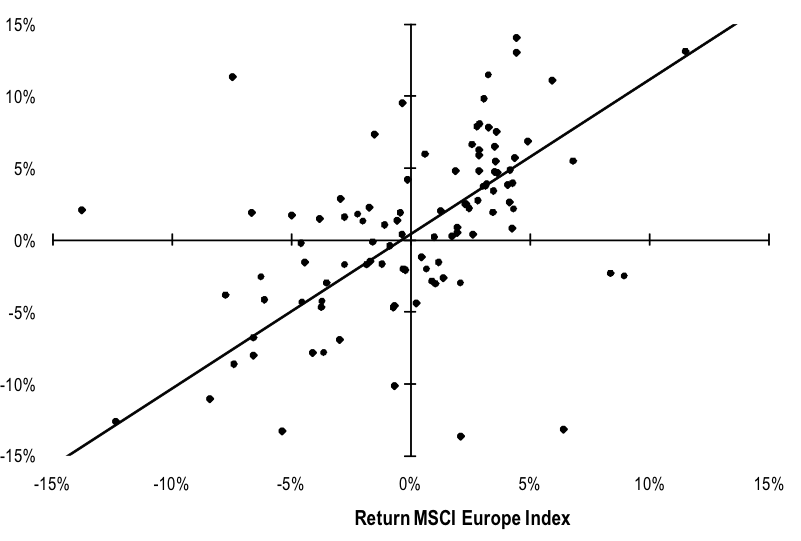
Loosely speaking, the regression fits a straight line through the observed returns as accurately as possible. The slope of this straight line is the beta estimate we are looking for.[1] The following figure provides an example. It graphically shows such a regression for the registered stock of Holcim using monthly data from January 2000 to June 2009. The market portfolio is approximated with the MSCI Europe Index. According to the numbers, the beta of Holcim registered stock is 1.07.
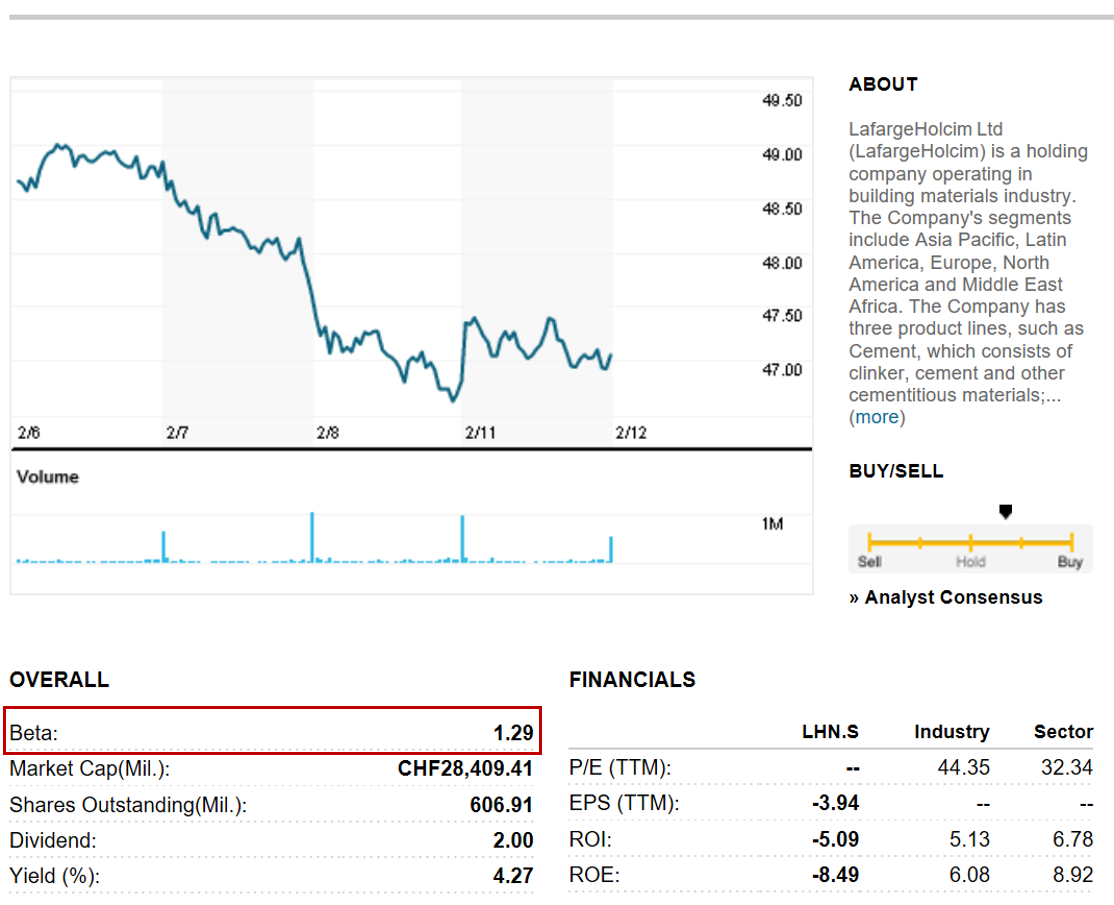
Another solution is to rely on the information provided by websites such as Google Finance, Yahoo Finance, Reuter, etc. In many instances, these websites provide acceptable estimates of beta as well.
In the case of Holcim, Reuters estimates a Beta of 1.29. Note, however, that this estimate was obtained in 2019 (10 years after the period considered in the regression above) and that Holcim had undergone a major merger with Lafarge in the meantime. Therefore, it is conceivable that the riskiness of the business has changed over time:
[1] Such betas are published in various financial publications or provided by various financial data services.