Reading: Startups as Real Options

The basic logic behind decision trees is both simple and convincing: Many things that we are uncertain about today will be known in the future. For exampe: Will our drug receive FDA approval? Will a plane that we develop fly? Will we strike oil when drilling in the desert? 

Decision trees attempt to systematically think through the future of a venture by forecasting major possible outcomes, assessing the probabilities of these outcomes, and then formulating possible reactions to these outcomes. 

Let's consider a simple example to illustrate decision trees and compare their outcome with the standard discounted cash flow (DCF) approach.

A company considers launching a new GPS tracking device for motorbikes. The required investment is 2 million today. According to the existing DCF analysis, the expected free cash flow of year 1 and year 2 is 1 million each. The relevant cost of capital is 10%. Based on this information, and assuming for simplicity that the firm only lasts 2 years, we could run a standard DCF valuation (in thousands):

Firm Value (DCF) = \( - 2'000 + \frac{1'000}{1.1}+ \frac{1'000}{1.1^2} = -264 \).

Based on our assumptions, it makes no sense to start this firm - the future cash flows cannot justify the required investment today.

However, what we have ignored in this valuation is managerial flexibility. Put differently, we did not really incorporate how the future expected cash flows come about. We have also assumed that the management will not adjust the project in year 2 in reaction to the learnings from year 1 and that the FCF of year 2 is independent from that of year 1. Let's look at this in some more detail.

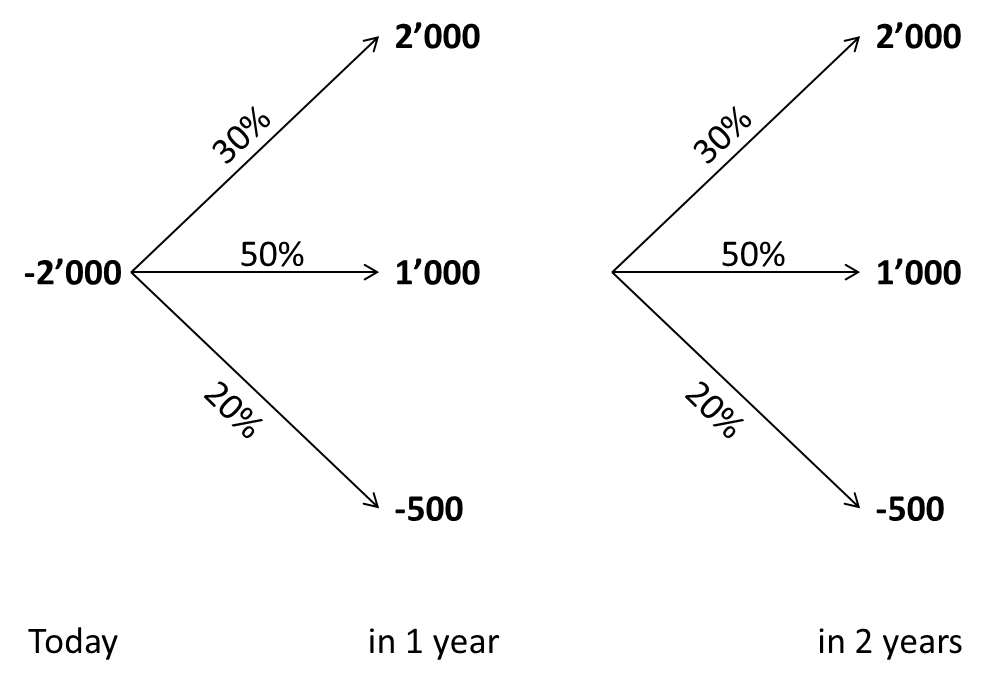
Let's assume that the cash flow estimate comes form three possible scenarios that the management deems realistic (values in thousands):

• Scenario 1: High demand for the product. In this case, the average FCF in 1 year is 2'000. The probability of this scenario is 30%.
• Scenario 2: Normal demand for the product. In this case, the average FCF in year 1 is 1'000. The probability of this scenario is 50%.
• Scenario 3: Low demand for the product. In this case, the average FCF in year 1 is -500. The probability of this scenario is 20%.

The expected cash flow of year 1 implied by the three scenarios is indeed 1 million (values in thousands):

Expected FCF = 0.3 × 2'000 + 0.5 × 1'000 + 0.2 × (-500) = 1'000

How could we try to incorporate management flexibility in the project and derive a decision tree?

From today's perspective, we do not yet know how the demand for the product will evolve. But this uncertainty will be partially resolved at the end of year 1. So why not put ourselves at the end of year 1 and think about how we would react in the tree possible outcomes (high, normal, low demand)? To illustrate, let's assume the following.

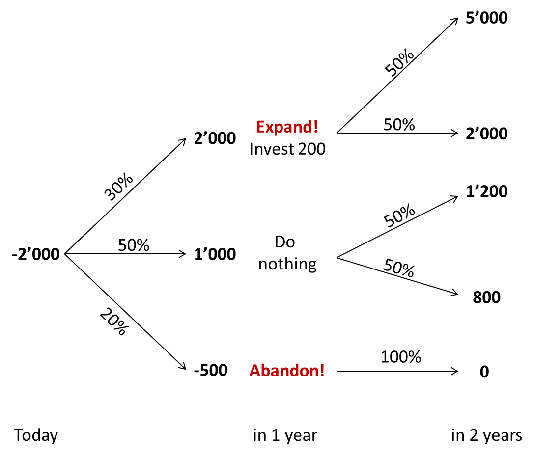
• High demand: If the management observes that there is high demand for the product, it expands production capacity and launches a second GPS tracking device that is targeted for bicycles. The required investment at the end of year 1 will be 200. In year two, the expected cash flows will then be either 5'000 or 2'000 with equal probability.
• Normal demand: If demand is normal, the management does not adjust the project. The expected cash flow of year 2 will then be either 1'200 or 800 with equal probability.
• Low demand: If demand is low, the project is abandoned. The expected cash flow of year 2 will therefore be 0.

With these additional considerations, we have tried to allow the management to learn about the product and its market environment and to react accordingly. Reacting means that the management exercises real options. In the project, we have incorporated two explicit real options: 

• The option to expand if demand is high
• The option to abandon if demand is low.

The decision tree in the following graph summarizes the revised project with the two real options. Arguably, such a decision tree could be a more realistic description of the project reality than what the standard DCF approach did.

The question now is: How to value such a tree?

Valuing the tree from today's perspective is rather complicated, as there are different branches with different probabilities and different numbers of sub-branches. Therefore, instead of starting the valuation from today's perspective, it is easier to value the tree step by step from the end to the beginning. This approach is also called backward-induction. Here is how it works:

• At the end of year 2, we will know exactly in which of the 5 possible states of the world we end up. 
• Now let's position ourselves one period earlier, at the end of year 1. At the end of year 1, we will know how the first year was and whether we ended up in the high, normal, or low demand scenario. So let's put ourselves in these respective scenarios at the end of year 1:
  • Low demand: In this case, the FCF of year 1 is -500. We abandon the project, so there are no other future cash flows. Consequently, the value of this scenario at the end of year 1 in this scenario is - 500:
     
    Value_{Low, 1} = -500 + 0 = -500
     
  • Normal demand: In this case, the FCF of year 1 is 1'000. In year 2, the FCF will be either 1'200 or 800 with equal probability. Hence, the value of this scenario at the end of year 1 is 1'909:
     
    Value_Normal,1 = \( 1'000 + \frac{0.5 \times 1'200 + 0.5 \times 800}{1.1}=1'909 \).
    
    
  • High demand: Finally, in the high-demand scenario, the firm generates a FCF of 2'000 at the end of year 1. At the same time, it also invests another 200. In year 2, the cash flow will then be either 5'000 or 2'000 with equal probability. Hence, the value of this scenario at the end of year 1 is
     
    Value_High,1 = \(2'000 - 200 + \frac{0.5 \times 5'000 + 0.5 \times 2'000}{1.1} = 4'982 \).

With these steps, we were able to determine the value of the project at the end of the first period. This value will be either -500, 1'909, or 4'982, depending on how the demand evolves during the first year. Consequently, we can simplify the above decision tree to:

This tree is now much easier to value from today's perspective. Given the assumed probabilities, the expected value of the project in year 1 will be 2.3 million:

Project value year 1 = 0.3 × 4'982 + 0.5 × 1'909 + 0.2 × (-500) = 2'349.

Given that today's investment is 2 million, the overall value of the firm, therefore, is 136'000:
 

Firm value = \( -2'000 + \frac{2'349}{1.1} = 136 \).

This example has shown how we can use decision trees to incorporate optionality into project or firm valuations. We d so step by step by simplifying the tree one period after the other.  In our particular case, the value of the option to expand and the option to abandon have increased the valuation of the investment opportunity from -264'000 with the "normal" DCF approach to 136'000 with a valuation approach that incorporates the optionality of the project.

Decision trees are a very powerful analysis tool and particularly helpful to study the management flexibility associated with major potential future developments. The problem with these trees is that they become very complex very quickly, since the world typically has more than 2 periods and 3 possible outcomes. Combined with this is, of course, the challenge to estimate all the values involved in a decision tree, including the cash flows in the various states, their probabilities, etc. Moreover, it is often not really clear what discount rates we should use to capitalize future cash flows.

Still, decision trees are the backbone of option pricing. Also the following two option pricing methods (binomial tree and Black-Scholes model) build on such trees. The trick will be to make some more restrictive assumptions about the structure of the tree to help us cut through the complexity.