Reading: Startups as Real Options

Suppose a company has an investment opportunity that it can realize within the next year. The required investment is 120 million. As of today, the present value of all future FCF the firm could generate with the investment is 100 million. Let's refer to this present value of all future FCF the "value of the underlying asset." Consequently, it does not make sense to invest today, as the NPV of the investment is -20 million:
 

NPV (investment today) = -Investment + PV(Future FCF) = -120 + 100 = -20 million.

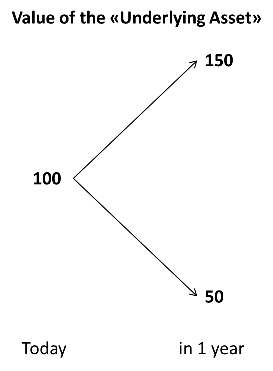
However, the company does not have to invest today. It can wait for 1 year and observe how the market for the product in question evolves. Let us assume that the value of the underlying asset can either increase to 150 or drop to 50. The following graph summarizes this value development:

How does this option to postpone the investment affect the analysis? While it does not make sense to realize the investment opportunity today, there is one future state of the world where the value of the underlying asset exceeds the necessary investment of 120 million:

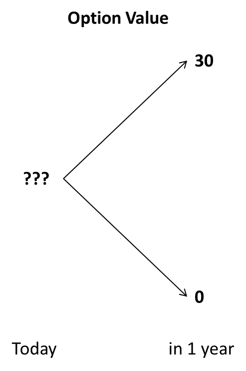
• If the value of the underlying asset goes up in 1 year, the investment of 120 million will unlock a future cash flow stream with a value of 150 million. Consequently, the NPV of the project in this particular state of the world will be 30 million in 1 year [= -120 + 150]. 
• In contrast, if the value of the underlying asset drops to 50 million in 1 year, it will not make sense to realize the project, as the NPV would be -70 million [= -120 + 50]. If we have the right to invest, but not the obligation, we will not invest and simply walk away. Consequently, in this scenario, the value of our right to invest will be 0.

The following graph summarizes the values of the investment opportunity that we have just derived.

As in the previous section, the question now is how to value this tree? We know that the value of the investment opportunity will be either 30 or 0 in 1 year. But we do not know the probabilities of these future state of the world! There, the graph with the value of the underlying asset comes in handy, as it implies the following:

• The current value of the underlying asset is 100
• The future value of the underlying asset is either 150 or 50.

If the asset pays no dividend, we know that the current value of the underlying asset (100) must correspond to the present value of the expected future value of the underlying asset (either 150 or 50 with unknown probabilities)! Let us denote the probability that the value of the underlying asset increases to 150 with the greek letter pi (π). Consequently, the probability that the value of the underlying asset drops to 50 is (1 - π). Therefore, the expected value of the underlying asset in 1 year is:
 

Expected value of underlying asset₁ = π × 150 + (1 - π) × 50 

Assuming that investors are risk neutral, we can discount this expected value at the risk-free rate of return (R) to get its present value:

PV(Expected value of underlying asset₁) = \( \frac{\pi \times 150 + (1-\pi) \times 50}{1+R} \).

We know that this expression must correspond to the current value of the underlying asset of 100:

100 = \( \frac{\pi \times 150 + (1-\pi) \times 50}{1+R} \).

So all we need to do is find the current risk-free rate of return to back out the implied probabilities of the future states of the world. Let's assume that the relevant risk-free rate of return (R) is 5%. Consequently:

100 = \( \frac{\pi \times 150 + (1-\pi) \times 50}{1.05} \).

Solving this expression for π implies that the probability of a value increase is 55%. Because we have assumed risk neutral investors (discounting at the risk-free rate of return), this probability is called the risk neutral probability. It is the probability that a risk neutral investor would attach to the scenario of a value increase. Why risk neutrality? The reason is that the "underlying asset" and the option that is written on this underlying asset generally do not have the same risk (the option is generally riskier than the underlying asset). Without risk neutrality, we could therefore not directly use the probabilities that are implied in the underlying asset value to price the option. 

If the risk neutral probability of a value increase is 55%, the corresponding probability of a value decline is 45%.

With these additional steps, we could back out the risk neutral probabilities of the future state of the world from the current asset prices. Now we know that there is a 55% probability of ending up in the high scenario and a 45% probability of ending up in the low scenario. This information we can now use to value our option!

• Remember that we have seen that the option value will be 30 million in the high scenario. Now we know that the probability of this outcome is 55%.
• Similarly, we learned that the option value will be 0 in the low scenario and that the probability of this scenario is 45%.

Consequently, we can write the expected option value in 1 year as:

Option value₁ = 0.55 × 30 + 0.45 × 0 = 16.5 million.

Under risk neutrality (risk-free discounting at 5%), the current value of the option, therefore, is 15.7 million:
 

PV(Option value₁) = 16.5/1.05 = 15.7 million.

This is, in all brevity, how we can value real options with binomial trees. The interesting takeaway is that the investment opportunity has a positive value (15.7 million) despit the fact that it does not make sense to invest today (NPV of -20 million). How is this possible? The investment opportunity gives us the RIGHT to invest today or in the future, but not the obligation. Put differently, we can wait and see how the value of the underlying asset evolves and then decide at a future point in time whether it makes sense to invest or not. The worst thing that can happen to us is that we do not invest and simply walk away. According to our calculations, this scenario has a probability of 45%. In this case, however, we do not lose any money. We simply don't invest.

In the next section, we formalize the notation of the above valuation steps so that it will be easier to apply in subsequent valuation situations.