Reading: Understanding and Valuing Debt and Equity

To value the constituents of the replicating portfolios, we have to be able to price two types of securities:

• Risk free bonds
• Options

This valuation idea goes back to a publication by Robert C. Merton in 1974, which is why it is generally referred to as the Merton model. The model is built on the assumption that the firm's debt in question is a zero-coupon bond, that is, it pays no interest during its lifetime and simply repays the notional amount at the time of maturity. To value a risk-free coupon bond, we therefore compute the present value of the notional amount (B), using the risk-free rate of return (R) as the discount rate.

Value risk-free bond = \( \frac{B}{(1+R)^{(T-t)}} \)

For example, a risk-free bond with a notional amount of 10 million that matures in 5 years has a current value of 9.06 million, assuming a risk-free rate of return of 2%:

Value risk-free bond = \( \frac{B}{(1+R)^{(T-t)}} = \frac{10}{1.02^5} \) = 9.06.

Valuing options is a bit more demanding. Here, we will rely on  the Black-Scholes valuation model. For a brief discussion of this model, and it's limitations in the context of firm valuation, please refer to the respective section in the course module Startup Valuation. The elegant aspect of the model is that, under a set of restrictive assumptions, the Black-Scholes model provides a closed-form solution to value options. According to the model, the value of an option (call and put) depends on the following 6 input parameters:

• V: The current value of the underlying asset. In our case, the firm value
• X: The exercise price of the option. In our case, the amount of debt outstanding
• T-t: The time to maturity. In our case, how long it takes for the debt to mature
• R: The risk-free rate of return. 
• Y: The dividend yield of the underlying asset. We assume, for simplicity, that the asset does not pay any dividends during the lifetime of the option and, therefore, set D = 0.
• σ: The volatility (standard deviation) of the return of the underlying asset. This is a measure of the riskiness of the asset.

The value of a call option (c) and a put option (p) can be derived using the following equations:

\( c = V \times e^{-y(T-t)} \times N(d_1) - X \times e^{-r(T-t)} \times N(d_2) \)

\( p = X \times e^{-r(T-t)} \times N(-d_2) - V \times e^{-y(T-t)} \times N(-d_1) \)

with:

• • \( r = ln(1+R) \)
     
  • \( y = ln(1+Y) \)
     
  • \( d_1 = \frac{ln(V/X)+(r-y+\sigma^2/2) \times (T-t)}{\sigma \times \sqrt{T-t}} \)
     
  • \( d_2 = d_1 - \sigma \times \sqrt{T-t} \)
     
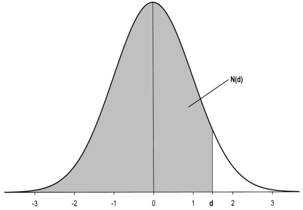
  • N(d.) = Probability that a standard normal variable is smaller than the value specified by d. It is the shaded surface under the standard normal distribution from -∞ to d.
     

For the purpose of this course, we should not worry too much about these equations. There are countless websites that help you apply them. For your convenience, we have also prepared a simple Excel file that does the necessary computations for you. It is available for download here.

Let's practice this valuation model with a simple example.