Reading: Towards an Optimal Capital Structure

In the real world, one of the main challenges is how to quantify the positive and negative implications of leverage. While the interest tax savings are fairly easy to quantify, the other side effects of financing are much harder to assess. For example, to what extent is the firm subject to managerial agency problems? Or how valuable is flexibility to the firm? Very often, the answer to these and similar questions cannot be summarized by an exact amount of money.

To better understand the trade-off between the costs and benefits of debt financing, firms (sometimes) use Monte Carlo Simulations. In what follows, we present a simplified case to find an optimal leverage range using Monte Carlo Simulations. The hypothetical firm we are considering has the following characteristics:

• The firm is expected to generate EBIT of 2'000 in year 1. Over the next 10 years, EBIT then increases by 5% each year.
• The firm's tax rate is 30%.
• Depreciation charges equal investments and the net working capital is not expected to change, so that the firm's free cash flow corresponds to NOPLAT [= EBIT × (1 - τ)].
• The firm's overall cost of capital (k_A) is 15%.
• The firm has currently no debt outstanding.

The following table summarizes the firm's expected cash flows over the next 10 years. 

 

	1	2	3	4	5	...	10
EBIT	2'000	2'100	2'205	2'315	2'431		3'103
- Taxes	600	630	662	695	729		931
NOPLAT	1'400	1'470	1'544	1'621	1'702		2'172
+ Depreciation	500	525	551	579	608		776
- Investments	500	525	551	579	608		776
- Change NWC	0	0	0	0	0		0
Free cash flow	1'400	1'470	1'544	1'621	1'702		2'172

  

Let's assume that there is uncertainty associated with the firm's EBIT. More specifically, we assume that the respective EBIT values have a "triangular distribution" with the following characteristics:

• The stated values in the table correspond to the most likely outcomes
• Each year, EBIT could be as low as 0 and as high as 1.5 times the most likely value

 

To illustrate, the following graph shows the theoretical distribution of year 5's EBIT:

 

 

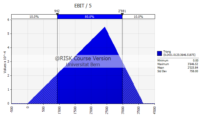
The shaded area in the graph represents the probability of various outcomes:

• According to our assumptions, EBIT will not drop below 0. Consequenly, negative EBIT values have zero probability.
• Similarly, we have assumed that EBIT will not be higher than 1.5 times the forecasted value, which is is 1.5×2'431 = 3'647. Consistent with this, the figure shows that the area for outcomes higher than 3'647 is empty.
• The peak of the distribution represents the most likely value of 2'431 (EBIT year 5, according to the table)
• The graph also shows that EBIT of year 5 will be below 942 in 10% of all cases and larger than 2'981 in 10% of all cases.

The EBIT of the other years are defined accordingly. 

 

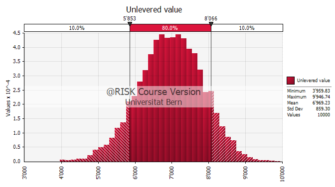
With this information, we can now conduct a simulation of the unlevered value of the firm. The outcome is summarized in the following graph. In short, our assumptions imply that the firm has an unlevered value of approximately 6'969. In 10% of the cases, the value could be 5'853 or lower, wherease in another 10% of the cases, the value could be 8'066 or higher. For a detailed description of how to conduct simulations in firm valuation, please refer to the module Coping with Measurement Error.

 

  

Let us now investigate how debt financing modifies the valuation. 

We assume that the firm can borrow at a rate of return (k_D) of 10%. In a first step, the following two considerations are relevant:

• Debt tax shield: The interest payments will lower the tax bill and improve firm value, accordingly.
• Cost of financial distress: If interest expenses exceed EBIT in any given year, we assume that the firm goes bankrupt and that the expected free cash flows drop to 0 for that year onwards.

 

To illustrate these two points, suppose the firm borrows 5'000 so that the annual interest payments are 500 [= 5'000 × 0.1]. The trade-off the firm faces is the following:

• If the annual EBIT exceed 500, the firm will benefit from tax savings of 150 [= 500 × 0.3] each year. Capitalized over 10 years at a cost of debt of 10%, these annual tax savings have a present value of roughly 922. This is the debt tax shield.
• The distribution of EBIT₅ in the above chart has shown, however that an EBIT of 500 cannot be guaranteed. In fact, according to the above chart, the probability is approximately 3% that EBIT₅ will be smaller than 500 and that the firm will therefore go bankrupt in that year. Bankruptcy implies that the cash flows of year 5 to year 10 drop to 0, so that firm value will be drastically reduced.

  

To solve the trade-off and find an "optimal" leverage range, we can run simulations similar to the one above with different debt levels. The result of such a simulation exercise is summarized in the following graph. The horizontal axis shows the amount of debt the firm borrows whereas the vertical axis shows the resulting mean expected value of the firm from a Monte Carlo Simulation similar to the one above. Without any debt outstanding, the value of the firm is 6'969, which is the value that we found in the preceding simulation.

 

 

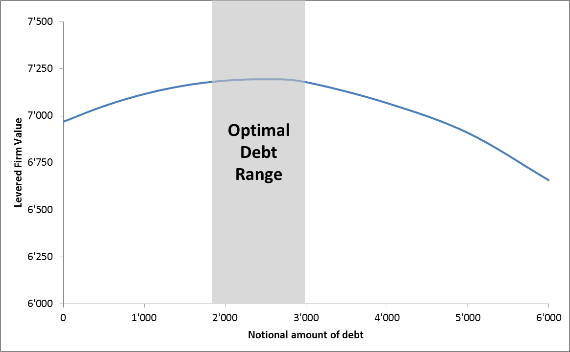
The main takeaways are as follows:

• Initially, firm value increases with additional borrowing. For example, at a debt level of 2'000, the estimated value is 7'188, which is roughly 3% higher than the unlevered value.
• Firm value will eventually drop if the company takes on too much debt. For example, at a debt level of 6'000, the estimated firm value is only 6'657, which is 4.5% below the unlevered value.
• Because the bankruptcy costs are quite material, it is not worthwhile for the firm to borrow a lot.
• Presumably, an optimal debt level for the company would be somewhere between 2'000 and 3'000 in this particular case, which corresponds to a debt ratio of roughly 35%.

 

Discussion

We have seen how we can in principle use Monte Carlo Simulation to assess the trade-offs between the costs and benefits of debt financing. In our particular case, the optimal debt ratio was approximately 35%.

Depending on how accurately we can measure the relevant factors and how costly it is for firms to adjust the capital structure, the optimal debt range will be broader or narrower. As long as the actual capital structure is within the optimal range, it is generally not worthwhile for firms to make adjustments, simply because the associated costs might not justify the benefits. Only when the firm's financing policy leaves the optimal range will it make sense for managers to act and bring leverage back to a value maximizing level. 

The optimal financing policy differs from firm to firm. According to Frank and Goyal (2009), there are six reliable factors that are correlated with cross-sectional differences in leverage:

• Median industry leverage: A firm tends to have a higher leverage if its industry peers are also highly levered. 
• Collateral / tangibility: Firms with significant collateral and more tangible assets tend to have higher leverage ratios.
• Size (log of assets): Large firms have comparatively higher leverage ratios than small firms. Presumably, large firms have better access to capital.
• Expected inflation: Leverage ratios are higher if expected inflation is high. All else the same, a higher expected inflation reduces the real cost of capital and therefore makes borrowing cheaper.
• Growth opportunities (Market-to-book ratio): Firms with significant growth opportunities have a comparatively lower leverage. Because they have comparatively few assets, these firms would have to borrow against cash flows, which might be unattractive. Moreover, high leverage might reduce their financial flexibility and thereby jeopardize the firm's growth options.
• Profitability: Finally, firms with high profits tend to have lower leverage ratios. 

 

Extension

These considerations, as well as the additional costs and benefits of debt that we have considered before, can be incorporated relatively easily into the above simulation analysis. This helps us illustrate how different firm characteristics change the theoretically optimal financing policy.

To see this, let us quickly go back to the previous example. There, we have assumed that the firm factually offers no collateral: In the case of bankruptcy, its value drops to 0. Clearly, this lowers a firm's debt capacity because the loss in default is very large.

Let us revisit the simulation from before under the assumption that the firm's assets will have a salvage value of 2'000 (instead of 0) in the case of bankruptcy. How does this affect our analysis? The following graph shows the results. The dashed blue line shows the debt-equity trade-off from the previous simulation whereas the red line replicates the simulation with the assumption that the salvage value is 2'000 in the case of default.

  

 

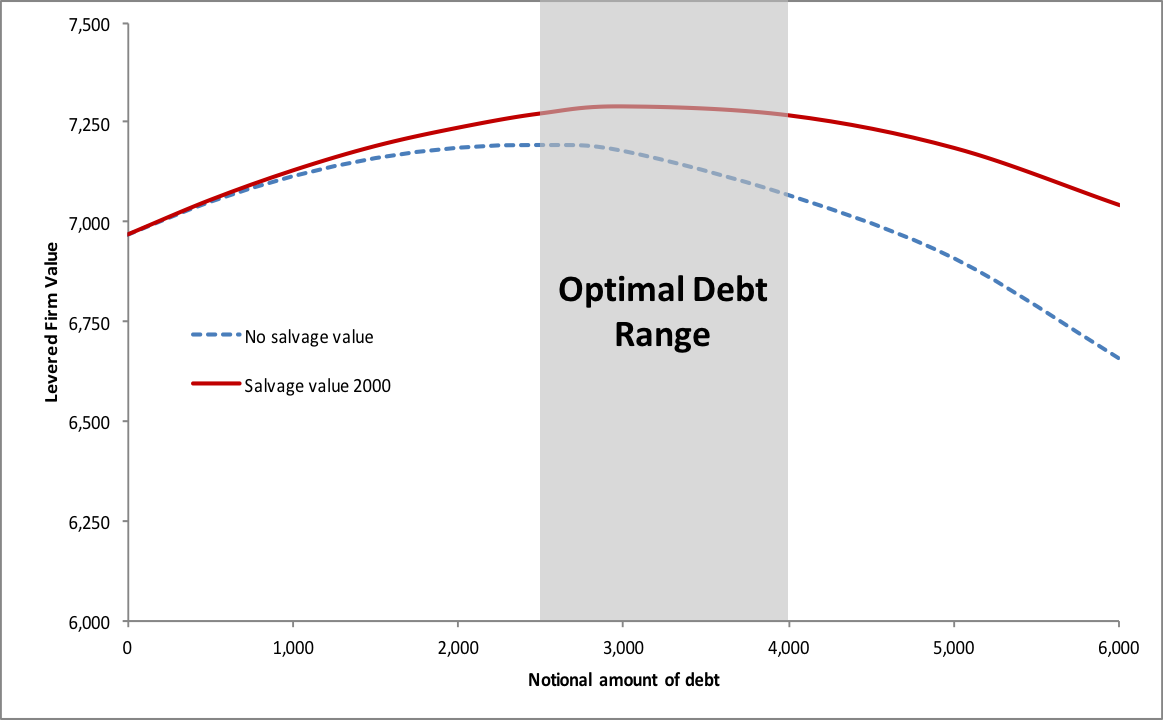
The main findings are as follows:

• Because of the salvage value of the firm's assets, the costs of financial distress become comparatively smaller. 
• Therefore, it takes a higher debt level for the cost of financial distress to outweigh the interest tax savings. 
• In our case, the optimal amount of debt would be somewhere between 3'000 and 4'000 (compared to a range of 2'000 to 3'000) in the previous simulation.
• Because the distress costs are comparatively smaller, firm value is comparatively larger. Around the optimal debt level, firm value would be close to 7'300 (compared to 7'150 from the previous simulation without salvage value).
• For the firm with collateral, the optimal debt ratio would therefore be in the neighborhood of 50% (compared to 35% before).

 

In line with the considerations from Frank and Goyal cited above, the simulation therefore shows that a firm with comparatively higher collateral should optimally borrow more than an otherwise identical firm with low collateral. The other side-effects of financing could be incorporated into the analysis in similar ways.