Reading: Return and Standard Deviation
4. Standard Deviation
Because the standard deviation is such an important risk measure, this section explains in more detail what a standard deviation is and how we can compute it. In brief, the journey will lead to the following equations:
\( \sigma^2 = \frac{1}{N-1} \sum_{i=1}^{N}(R_i-\mu)^2 \)
\( \sigma = \sqrt{\sigma^2} = \sqrt{\frac{1}{N-1}\sum_{i=1}^{N}(R_i-\mu)^2}\)
with:
| \(\sigma\) | Standard deviation (Volatility) |
| \(\sigma^2 \) | Variance (squared volatility) |
| \(\mu\) | Average (mean) expected return |
| \(R_i\) | Return of year i |
| \(N\) | Number of observations (years) |
The good news is that for real-world applications, we will not have to make these cumbersome calculations by hand. There are built-in functions in Microsoft Excel that take care of this, in particular the function "=STDEV()". Still, it is useful to understand what is actually going on when we use this function. Let us illustrate this with a relatively simple example.
Example: Standard deviation of equity returns 2014-2018
To practice the computation of a standard deviation, let us look at the last five years of equity returns from the previous page, i.e., the years 2014 - 2018:
The average return (\(\mu\))
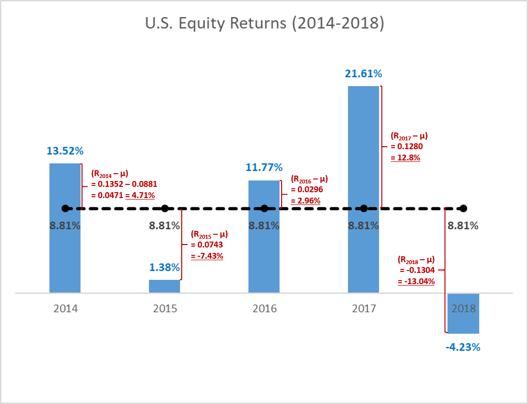
- The blue bars in the graph show the actual annual U.S. equity returns of the five years under investigation. For example, in 2014, the return was 13.52%. In keeping with our notation above, we denote this return R2014 = 0.1352.
- The dashed black line shows the average return \(\mu\) (arithmetic mean) over the five years. During that period, the average return \(\mu\) was 8.81%. We find this average as follows:
\( \mu = \frac{R_{2014}+R_{2015}+R_{2016}+R_{2017}+R_{2018}}{5}\) \(=\frac{0.1352+0.0138+0.1177+0.2161-0.0423}{5}\) \(=0.0881 = 8.81\%\)
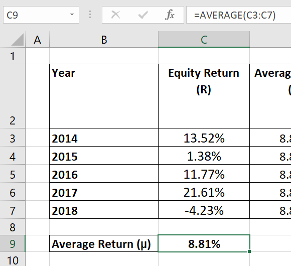
In the accompanying Excel file, the returns of the individual years are in cells C3 to C7. Using these returns, cell C9 calculates the average return by using the function =AVERAGE(C3:C7):
Deviation from the mean
With this information, we are now ready to compute by how much the individual returns (\(R_i\)) deviate from the average (\(\mu\)). For example, in 2014, the return was 13.52%, which is 0.0471 higher than the average of 8.81%:
\(R_{2014} - \mu = 0.1352-0.0881 = 0.0471 = 4.71\% \)
The red calculations in the return graph above replicate this procedure for all 5 years under investigation. For example, in 2015, the equity return (\(R_{2015}\)) deviated by -7.43% from the mean and in 2018, the deviation was -13.04%.
Now remember that we are looking for the Standard deviation, that is, the "typical" deviation of our returns from the mean. The initial reaction could be to simply take the average of the individual annual return deviations that we have just computed. Unfortunately, that does not work, as the positive and negative deviations will perfectly offset each other, so that the average deviation from the average is zero (after all, that's the definition of the average…).
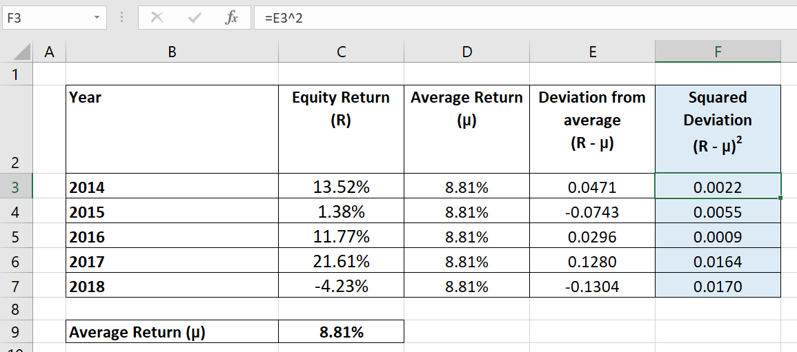
As a workaround, we can square the individual deviations in order to obtain all positive values. For example, in 2014, the squared deviation from the mean is 0.0022 and in 2018, the squared deviation from the mean is 0.0170:
\((R_{2014} - \mu)^2 = (0.1352-0.0881)^2 = 0.0471^2 = 0.0022 \)
\((R_{2018} - \mu)^2 = (-0.0423-0.0881)^2 = -0.1304^2 = 0.0170 \)
The following screenshot from the accompanying Excel file shows the result of this procedure for all 5 years in column F:
Variance and Standard Deviation
Now we are almost done... Looking at the original equation for the variance, what remains to be done is to take the sum of the individual squared deviations \(\sum_{i=1}^{N}(R_i-\mu)^2 \) and to divide the result by \((N-1)\).
Based on the numbers above (column F of the Excel file), the sum of the squared deviations is 0.0420:
\(\sum_{i=1}^{N}(R_i-\mu)^2 = 0.0022+0.0055+0.0009+0.0164+0.0170 = 0.0420 \)
By dividing this value by the number of returns minus 1 \((N-1) = 5-1=4\), we finally get the variance of the returns \((\sigma^2)\) of 0.0105:
\( \sigma^2 = \frac{1}{N-1} \sum_{i=1}^{N}(R_i-\mu)^2 =\frac{0.0420}{5-1}=0.0105\)
To obtain the standard deviation (volatility, \(\sigma\)), we now take the square root of the variance and find a volatility of 10.25%:
\( \sigma = \sqrt{\sigma^2}=\sqrt{0.0105} = 0.1025 = 10.25\% \)
After all these calculations, we are finally able to characterize the distribution of the annual U.S. equity returns between 2014 and 2018: The average annual return during that time was 8.81%, with a standard deviation of 10.25%.
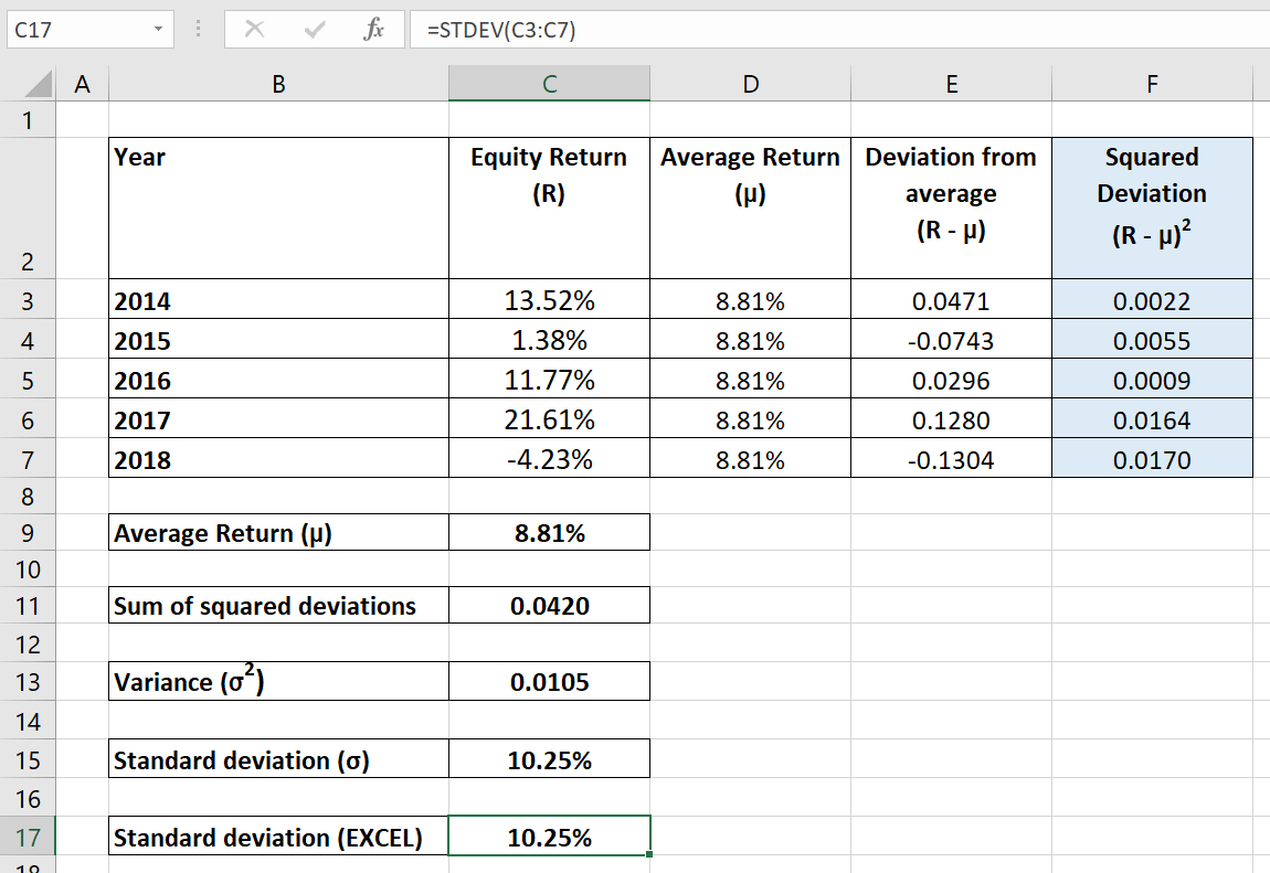
This example has shown step-by-step how to compute the standard deviation of a series of returns (or any other values). As we have already mentioned at the beginning, there is a convenient Excel function that takes care of all these steps: =STDEV(). This function is implemented in cell C17 of accompanying Excel file. To compute the standard deviation of the return series (cells C3 to C7), all we have to do is enter
=STDEV(C3:C17).
As the following screenshot shows, the result is the same as before, a standard deviation of 10.25%. Therefore, it seems that Excel knows how to compute standard deviations...