Reading: Introduction to Diversification
4. A Portfolio with Two Assets
Let us now generalize the computation of the expected return and standard deviation of a portfolio. We start with a portfolio P that contains two assets. Let's use the generic names A and B for the two assets (going back to our initial example, A could be equities and B could be bonds).
The key equations to compute the average expected return (\(\mu_P\)) and the standard deviation of the return (\(\sigma_P\)) of a portfolio with two assets A and B:
Average Expected Portfolio Return (\(\mu_P\))
\( \mu_P = w_A \times \mu_A + w_B \times \mu_B \),
with \(\mu\) = average expected return; w = portfolio weights; P = portfolio; A and B = portfolio constituents. If we assume that all the money is invested, \( w_A + w_B = 1\). Therefore, \(w_B = (1-w_A)\). Consequently, the above expression simplifies to:
\( \mu_P = w_A \times \mu_A + (1-w_A) \times \mu_B \).
In words: The average expected portfolio return corresponds to the weighted average expected return of the individual assets inside the portfolio (A and B, in our case).
Return Variance and Standard Deviation (\(\sigma_P^2; \sigma_P\))
The computation of the return variance is a bit more complex, namely:
\( \sigma^2_P = w_A^2 \times \sigma_A^2 + (1-w_A)^2 \times \sigma_B^2 + 2 \times w_a \times (1-w_A) \times \rho_{AB} \times \sigma_A \times \sigma_B \)
where \(\sigma^2\) is the return variance (squared standard deviation \(\sigma\)) and \(\rho\) denotes the correlation between the returns of assets A and B.
The term \(\rho_{AB}\times \sigma_A \times \sigma_B \) is the so-called covariance of the returns of assets A and B. This covariance is denoted as \(\sigma_{AB}\):
\(\sigma_{AB} = \sigma_A \times \sigma_B \times \rho_{AB} \)
Therefore, the above expression of the portfolio variance can also be written as:
\( \sigma^2_P = w_A^2 \times \sigma_A^2 + (1-w_A)^2 \times \sigma_B^2 + 2 \times w_a \times (1-w_A) \times \sigma_{AB} \)
To obtain the standard deviation of the portfolio return (\(\sigma_P\)), we take the square root of the variance:
\(\sigma_P = \sqrt{\sigma_P^2} \).
These are the most important formulas we need to compute the risk and return of a portfolio.
Example: U.S. Stocks and Bonds
To practice these equations, we go back to the example of U.S. stocks and bonds over the years 1928-2018. From before, we already know the average return and standard deviation of the two assets:
| U.S. Stocks (Asset A) |
U.S. bonds (Asset B) |
|
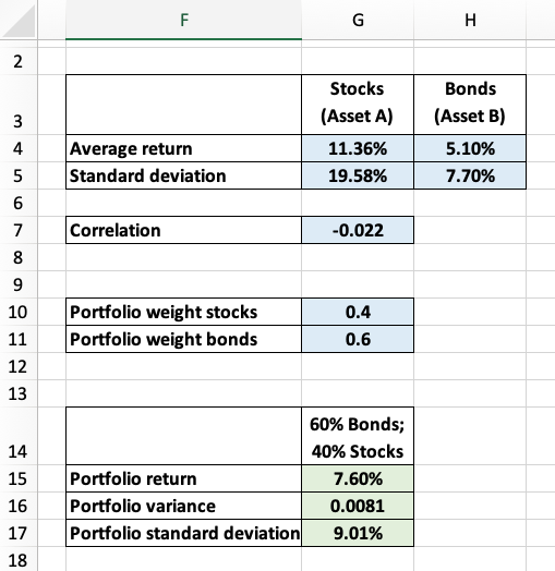
| Average annual return (\(\mu\)) | 11.36% | 5.10% |
| Standard deviation (\(\sigma\)) | 19.58% | 7.70% |
Moreover, in the section on the return distribution, we have seen, but not yet discussed, that the correlation between the two return series (\(\rho\)) is −0.022.
Let us now compute the risk and return of a portfolio that allocates 40% of the money to stocks and 60% of the money to bonds. In keeping with the notation above, we call the stocks "Asset A" and the bonds "Asset B."
Portfolio return: 40% stocks (Asset A) 60% bonds (Asset B)
Based on our assumptions, the average expected return of the portfolio is 7.60% p.a.:
\( \mu_P = w_A \times \mu_A + (1-w_A) \times \mu_B \) \( = 0.4 \times 0.1136 + 0.6 \times 0.0510 = 0.0760 = 7.60\% \).
Portfolio volatility: 40% stocks (Asset A) 60% bonds (Asset B)
The same portfolio has a volatility (return standard deviation) of 9.01%. Specifically, the return variance is 0.0081:
\( \sigma^2_P = w_A^2 \times \sigma_A^2 + (1-w_A)^2 \times \sigma_B^2 + 2 \times w_a \times (1-w_A) \times \rho_{AB} \times \sigma_A \times \sigma_B\) \(= 0.4^2 \times 0.1958^2 + 0.6^2 \times 0.0770 + 2 \times 0.4 \times 0.6 \times 0.1958 \times 0.0770 \times (-0.022)= 0.0081\)
Consequently, the standard deviation of the portfolio return is 9.01%:
\( \sigma_P = \sqrt{\sigma_P^2} = \sqrt{0.0081} = 0.0901 = 9.01\%\).
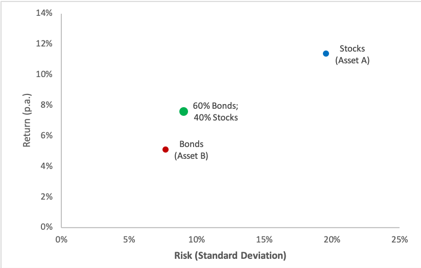
Therefore, a portfolio that invests 40% in U.S. stocks and 60% in U.S. bonds has an average return of 7.60% and a volatility of 9.01%.
When we plot this portfolio in the risk-return diagram from before (green dot), we see that most of the extra risk of stocks has disappeared, while the average return of the portfolio is considerably higher than that of bonds. Diversification therefore does indeed seem to help investors optimize the risk-return profile.
For ease of application, the worksheet "2 Assets Portfolio" of the enclosed Excel file contains the Excel-implementation of these computations:
- In cell G10, enter the portfolio weight of stocks (\(w_A = 40\%\));
- Cell G15 then shows the average portfolio return (\(\mu_P = 7.60\%\));
- Cell G17 shows the standard deviation of the return (\(\sigma_P = 0.901\)).