Reading: Portfolio with Multiple Assets
2. Efficient Frontier
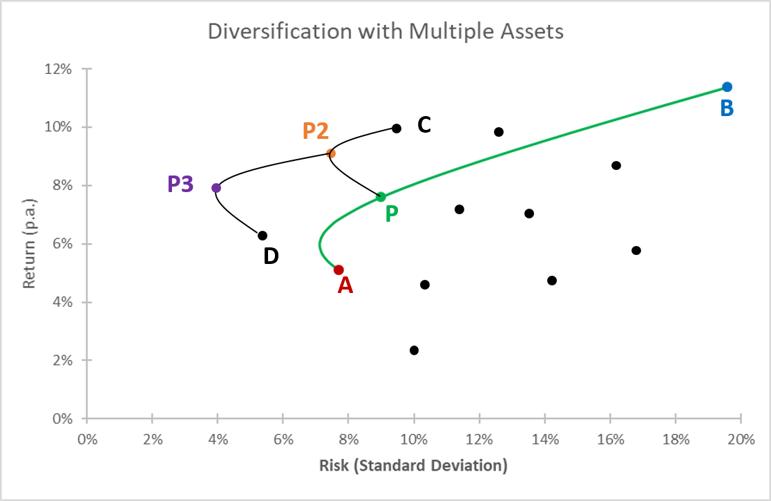
In principle, diversification with multiple assets simply replicates the procedure from the 2-assets world with many different combination of asset pairs. Here is the basic logic, which is also summarized in the graph below:
- In the two-asset world, we have combined asset A and asset B into a portfolio P. And we have computed the average return and standard deviation of that portfolio.
- Now let us suppose that there are many other assets out there, whose risks and returns are characterised by the black dots in the graph below.
- We could now take the portfolio P from the first step and combine it with, say, asset C. This brings us back to the two-asset case, so we know how to compute the risk and return of any combination between the two assets P and C. Let's suppose the desired combination is P2.
- Then we take the resulting portfolio P2 and, again, combine it with an asset, say D. The result of the portfolio formation could be portfolio P3, which is shown in purple in the graph below.
We can repeat this procedure until we find the portfolio with the ideal risk-return combination. In doing so, the key question is to what extent we can diversify the existing risk. As we have seen in the two-asset case, the correlation between the assets sets the limit to diversification. Perfect risk diversification is only possible if we find assets with perfect negative correlation. Unfortunately, these assets do not exist in the real world. Therefore, in the real world, there is a limit to risk diversification: If we want to earn a certain rate of return, we have to accept some risk that cannot be diversified any further.
The following figure illustrates these limits to diversification with the red hyperbola. For any given rate of return (vertical axis), it shows the portfolios that achieve this return with the lowest possible risk (horizontal axis). Therefore, the hyperbola is called the minimum standard deviation of return frontier.
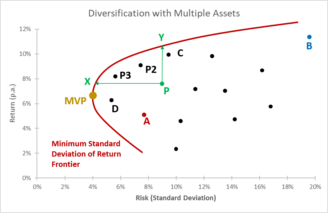
The portfolios that are on the frontier are called efficient portfolios: They offer a given rate of return at the lowest possible risk.
The portfolios that are inside the frontier are called inefficient portfolios: With additional diversification, investors could achieve a better risk-return pattern. For example, take the portfolio P: With additional diversification:
- The same rate of return (approximately 8%) could be achieved with a much lower risk (approximately 4% instead of 9%). The portfolio that offers the same rate of return as P at the lowest possible risk is portfolio X.
- Alternatively, with the same amount of risk (approximately 9%), investors could earn a much higher return. The portfolio with the highest possible return, given the risk, is portfolio Y on the minimum standard deviation frontier.
Portfolios X and Y, and all portfolios in between on the minimum standard deviation frontier, clearly dominate portfolio P in terms of the risk and return patter that they offer. Proper diversification therefore helps investors to earn higher returns at a lower risk.
The last point on the minimum standard deviation frontier that is worth noting is the Minimum Variance Portfolio (MVP). This portfolio to the very left shows the combination of risky assets that leads to the lowest possible risk. That's as safe as an investment can get if we decide to put money in risky assets to begin with.
The Minimum Variance Portfolio is also a very important portfolio because it marks the starting point of all portfolios that lie on the upward-sloping segment of the minimum standard deviation frontier, the so-called Efficient Frontier.
- Risk averse investors will not choose a portfolio that lies in the downward-sloping segment of the frontier (to the bottom right of the MVP), as these portfolios offer a inefficiently low return for a given level of risk.
- Because investors will only pursue portfolios to the upper right of the MVP, the upward sloping segment of the frontier is the Efficient Frontier.
The following graph shows the efficient frontier. If we limit our investment universe to risky assets, the efficient frontier denotes the set of portfolios with the best possible risk-return characteristics.

The logical next step is to see how the investment universe changes when we introduce a risk free asset. This will be the next, and last, major step of the discussion.