Reading: Portfolio with Multiple Assets
4. Portfolios with Riskless Borrowing and Lending
So far, all the assets that we have considered exposed the investor to risk. Graphically speaking, all assets were to the right of the vertical axis in the risk-return space (because they have risk).
How does the picture change when we introduce a risk-free asset to our investment opportunities? As the name already suggests, a risk-free asset guarantees a certain rate of return over a specified investment period. In our risk-return graph, the risk-free asset therefore lies on the vertical axis (some given return; no risk).
For example, in February 2019, U.S. Treasury Bonds promised an average annual rate of return of 2.65% over the next 10 years. If we buy the bond in February 2019, hold it until maturity 10 years later, and assume that the U.S. government does not go bankrupt in between, we will earn an average annual return of 2.65% with certainty. (Note that during the investment period, returns will fluctuate, depending on the changes in the term structure of interest rates).
How does the availability of such a risk-free asset change the investment opportunity set? Let us take a look.
Portfolios with risk-free asset
For simplicity, let us assume that we can choose between stocks (as before, with a return of 11.36% and a standard deviation of 19.58%) and the risk-free asset, which we assume to generate an annual rate of return of 2.65% over the next 10 years.
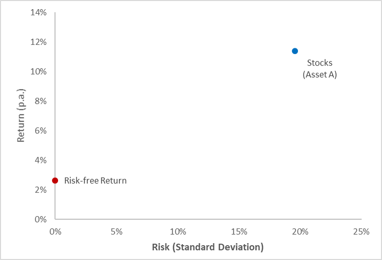
The following diagram plots the two assets:
- If we invest all our money in stocks, we end up in the blue spot.
- Alternatively, if we invest all our money in the risk-free asset, we end up in the red spot.
The tricky question now is: What happens if we invest in both stocks and the risk-free asset?
We can answer this question with the knowledge from the previous section on diversification with 2 assets. To do so, we need the necessary information about risk, return, and correlation:
| Stocks (Asset A) |
Risk-free asset (Asset R) |
|
| Mean return (\(\mu\)) | 11.36% | 2.65% |
| Standard deviation (\(\sigma\)) | 19.58% | 0.00% |
| Correlation between returns (\(\rho_{AR}\)) | 0.00 | |
Importantly, the correlation between the risk-free asset and any risky asset is zero: Because the risk-free return does not change, the price movements of risky assets must be unrelated to the risk-free asset.
Now that we have all the ingredients, we can compute the risk and return of a portfolio that invests in both assets. Let us assume that we invest 30% of the capital in stocks (\(w_A = 0.3\)) asset and 70% in the risk-free asset (\(w_R = 0.7\)).
Using the equations from before, the return and risk of the resulting portfolio are:
As before, the portfolio return \(\mu_P\) is a weighted average of the returns of stocks and the risk-free rate. Allocating 30% to stocks and 70% to the risk-free asset, the resulting portfolio return is 5.26%:
\(\mu_P = w_A \times \mu_A + w_R \times \mu_R \) \(= 0.3 \times 0.1136 + 0.7 \times 0.0265 = 0.0526 = 5.26\%\)
The variance of the portfolio is:
\(\sigma^2_P = w_A^2 \times \sigma_A^2 + (1-w_A)^2 \times \) \(\sigma_R^2 +2 \times w_a \times (1-w_A)\times \rho_{AR} \times \sigma_A \times \sigma_R \)
Since the risk-free asset has zero volatility and variance (\(\sigma_R = \sigma_R^2 = 0\)) and is uncorrelated with the risky asset (\(\rho_{AR}=0\)), this expression simplifies to:
\(\sigma^2_P = w_A^2 \times \sigma_A^2\).
Consequently, the volatility of a portfolio the portfolio with (\(1-w_A\)) allocated to the risk-free asset is:
\(\sigma_P = \sqrt{w_A^2 \times \sigma_A^2} = w_A \times \sigma_A\).
In our case, the portfolio volatility therefore is 5.87%:
\(\sigma_P = \sqrt{w_A^2 \times \sigma_A^2} = w_A \times \sigma_A = 0.3 \times 0.1958 = 0.0587 = 5.87\%\).
The following diagram depicts the resulting portfolio in the risk-return space (green dot):
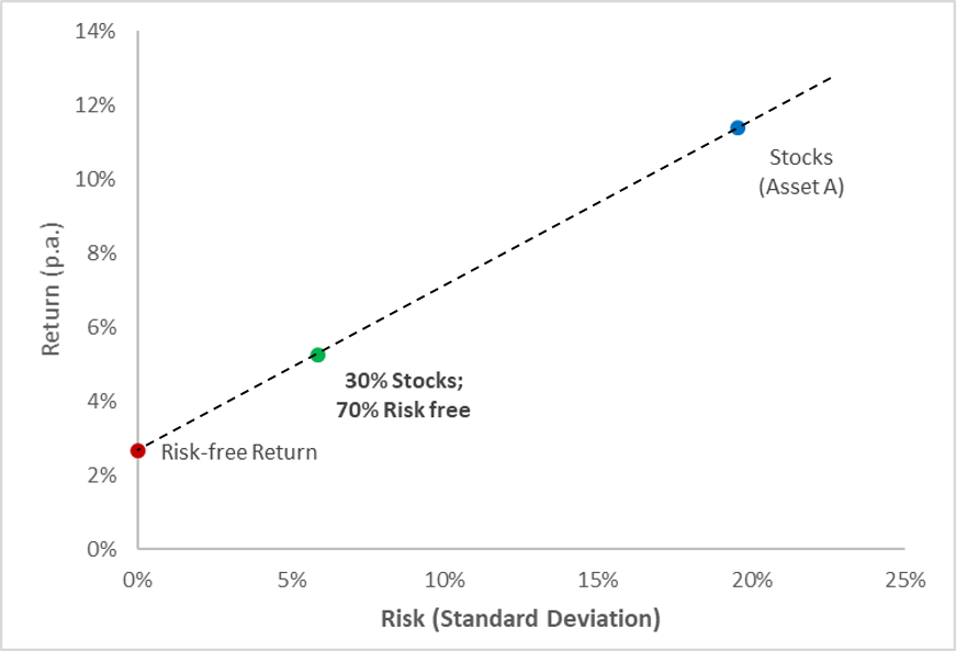
The portfolio lies on a straight line that connects the risk-free asset and the risky asset in the risk-return space. This statement can be generalized:
Whenever we combine a risky asset with the risk free asset, the resulting portfolios lie on a straight line that goes through both the risky and the risk-free asset.
As we see in the graph above, the dashed line actually extends beyond the blue dot that demarks the risky asset (stocks). How is this possible? Remember what the line shows:
- As we move to the right of the dashed line, we allocate an increasing fraction of our wealth to the risky asset.
- In the blue dot, 100% of our wealth is invested in stocks.
- To go beyond the blue dot, we have to invest more than 100% in stocks! We can do so by borrowing money at the risk free rate and invest the proceeds in the risky asset!
Technically speaking, the portfolios that are to the right of the risky asset have \(w_A > 1\) and therefore \( w_B < 0\). They are called levered portfolio, because they use leverage to increase the expected rate of return (and risk).
Example:
Let us assume that we want to invest 130% of our money in the risky asset (\(w_A = 1.3\)). In order to do so, we have to borrow (\(w_B = 1-w_A = 1-1.3=-30\%\)) at the risk-free rate. Using the equations from above, the return and standard deviation of the resulting portfolio are 13.97% and 25.46%, respectively:
\(\mu_P = w_A \times \mu_A + w_R \times \mu_R \) \(= 1.3 \times 0.1136 -0.3 \times 0.0265 = 0.1397 = 13.97\%\)
\(\sigma_P = w_A \times \sigma_A =1.3 \times 0.1958 = 0.2545 = 25.46\%\).
When we plot this levered portfolio in the risk-return space (golden dot), we see that it does indeed lie on the straight line that connects the risk-free asset and the risky asset. But it is to the upper right of the risky asset, meaning that it is expected to generate a higher return than the risky asset (at a higher risk):
This graph, and the underlying discussion, has crucial implications:
- First, whenever we combine a risky asset with the risk-free asset, the resulting portfolios are on a straight line that goes through both assets. This essentially leaves one question unanswered: with which risky asset shall we combine the risk-free asset? This question will be answered next.
- Second, we got an impression of the power of leverage. To earn a higher return, we do not necessarily have to look for assets with a high return. We can also use a less risky asset (in our case stocks) and borrow against this asset! Once we understand this, we can, in principle, combine portfolios with any expected rate of return! The sky is the limit (however also in terms of risk).