Reading: Capital Asset Pricing Model (CAPM)
2. Capital Asset Pricing Model
The discount rate is the average rate of return that investors expect earn when investing in a given asset (project). In the context of portfolio diversification, we have referred to this average expected return as \(\mu\).
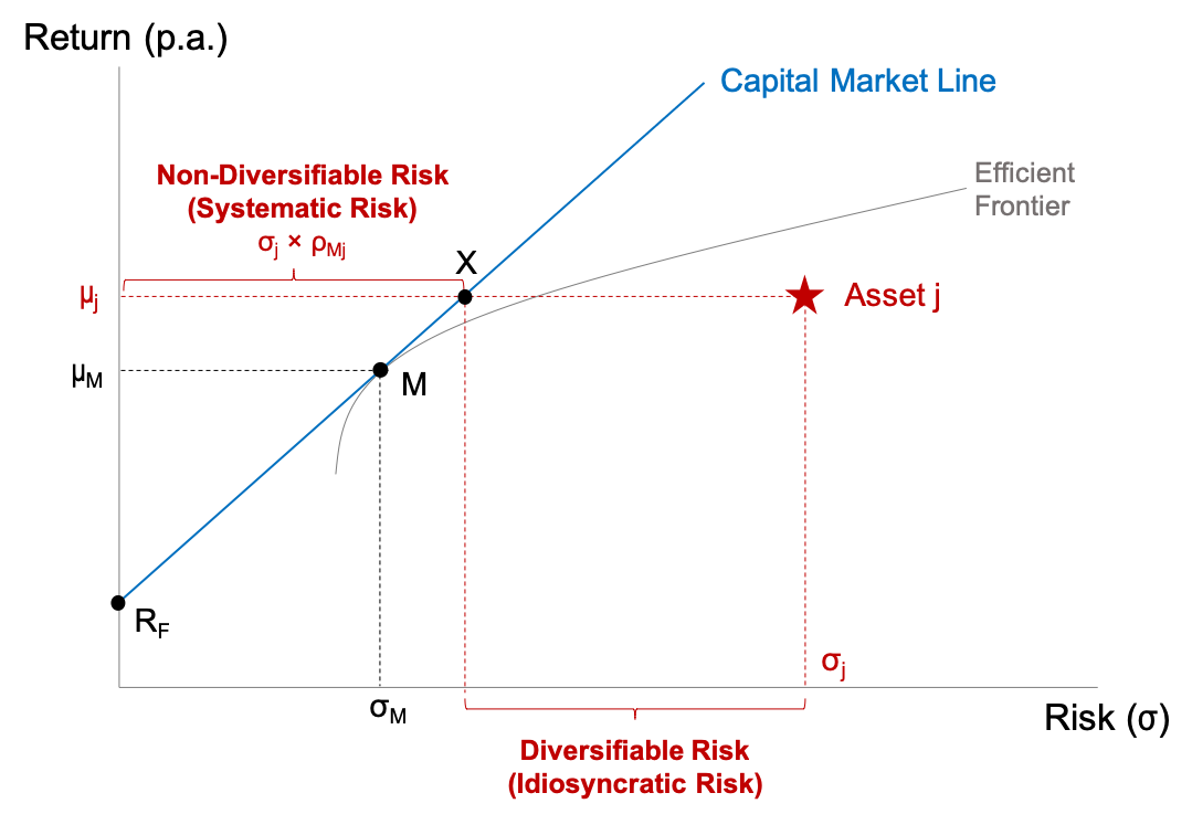
Our goal is to establish a relationship between the average rate of return of asset j (\(\mu_j\)), the riskiness of that asset, as well as the risk and return characteristics of the market portfolio. All these elements are depicted in the graph below, which was developed in detail in the section on the Capital Market Line and the Market Portfolio:
To structure the discussion, let us assume the following scenario, which corresponds to the typical situation faced by financial managers who want to estimate discount rates:
- We want to determine the average expected return of asset j, \(\mu_j\). We do not know that return yet.
- However, we have information about the riskiness of the asset (\(\sigma_j\)), the risk and return of the market portfolio (\(\sigma_M; \mu_M\)), the risk-free rate of return (\(R_F\)), as well as the correlation between the returns of asset j and the market portfolio (\(\rho_{Mj}\)).
To make things more concrete, let's assume the following values for these parameters:
| Variable | Description | Value |
| \(R_F\) | Risk-free rate of return | 2.00% |
| \(\mu_M\) | Average return on market portfolio | 7.00% |
| \(\sigma_M\) | Volatility of market portfolio | 15.00% |
| \(\sigma_j\) | Volatility of asset j | 45.00% |
| \(\rho_{Mj}\) | Correlation between the two returns | 0.50 |
What does all this information tell us about the expected return on asset j?
Let's tackle this question step by step.
(1) First, let us ignore asset j for a moment and focus on the market portfolio (M) instead:
- Investors who buy the market portfolio are exposed to a volatility of 15%, as per our assumptions (\(\sigma_M = 15\%\)).
- Remember from our discussion before, that the market portfolio is perfectly diversified. Put differently, it offers the highest possible return for a volatility of 15%. The risk of the market portfolio is therefore purely systematic risk.
- For this systematic risk, the market portfolio is rewarded with an average return of \(\mu_M = 7\%\), which is 5% higher than the risk-free rate or return (\(R_F = 2\%\)). This return spread between the market portfolio and the risk-free rate is the so-called Market Risk Premium (MRP):
Market Risk Premium (MRP) = μM − RF = 0.07 − 0.02 = 5.00%
- Therefore, we have established that investors require a risk premium of 5% over the risk-free rate when holding the market portfolio with a systematic risk of \(\sigma_M\) = 15%.
(2) Second, we define the market portfolio as our relevant risk benchmark: Put differently, we measure the risk of all other assets relative to the risk of the market portfolio.
- Assets with the same systematic risk as the market portfolio will earn the same risk premium as the market portfolio.
- Assets with a larger systematic risk will earn a larger risk premium than the market portfolio. For example, if the systematic risk of an asset is twice the systematic risk of the market, the asset should earn a risk premium of twice the market risk premium, i.e., 10% in our example.
- In contrast, assets with a smaller systematic risk will earn a smaller risk premium than the market. For example, if an asset is half as risky as the market, it should earn a risk premium equal to half the market risk premium.
In our original equation to determine the appropriate discount rate, the "Price of Risk" consequently is the market risk premium (MRP) whereas the "Amount of Risk" is the asset's systematic risk relative to the market risk. This risk measure is the so-called "Beta", β, of the asset:

Consequently, the last remaining item that we have to discuss is the risk measure beta (β), the risk of asset j relative to the market risk.
(3) Third, we determine how risky asset j is compared to the market portfolio.
- According to our assumptions, the volatility of asset j (\(\sigma_j\)) is 45% whereas volatility of the market (\(\sigma_M\)) is 15%. Our initial conclusion could therefore be that asset j is three times as risky as the market, which is why it should earn a risk premium equal to three times the market risk premium.
- However, the discussion about portfolio diversification has shown that the volatility of an individual asset is an inappropriate risk measure. The reason is that investors who add this asset to a well-diversified portfolio will be able to diversify part of that risk.
- In the graph above, we see that investors who hold asset j can eliminate a considerable part of asset j's risk through diversification. In the graph, diversification allows investors to move from asset j to the point X on the Capital Market Line. The risk difference between X and j is therefore called diversifiable risk (idiosyncratic risk). Because investors can easily eliminate this risk with diversification, it is not rewarded with a higher rate of return.
- The remaining risk, however, cannot be diversified. The distance between X and the vertical axis is the non-diversifiable or systematic risk of asset j. This is the risk that asset j contributes to a well-diversified portfolio. For this risk, investors need to be rewarded with a higher expected rate of return.
- As it turns out, the systematic risk of an asset corresponds to the volatility of the asset (\(\sigma_j\)) times the correlation of the asset with the market (\(\rho_{Mj}\)):
Systematic Riskj = \( \sigma_j \times \rho_{Mj} \)
- In our example, the volatility of j (\(\sigma_j\)) is 45% and the correlation with the market (\(\rho_{Mj}\)) is 0.5. Therefore, the systematic risk of asset j, is 22.5%:
Systematic Riskj = \( \sigma_j \times \rho_{Mj} = 0.45 \times 0.5 = 0.2250 = 22.5\%\)
- Put differently, the systematic risk of asset j is 1.5 times the systematic risk of the market portfolio. 1.5 therefore is the beta of asset j:
\(\frac{\text{Systematic Risk}_j}{\text{Market Risk}} = \frac{\sigma_j \times \rho_{Mj}}{\sigma_M} = \frac{0.225}{0.150} = 1.5 = \beta_j \)
- This is the famous beta. And the idea behind it is quite simple: The systematic risk of an asset is measured relative to the risk of a benchmark portfolio—the market portfolio. Beta is the most prominent (and the most heatedly discussed) risk measure among finance professionals.
Putting it all together
With all these analyses, we are (finally) ready to compute the average expected return on asset j (\(\mu_j\)):
\( \mu_j = R_F + \beta_j \times MRP = 0.020 + 1.5 \times 0.05 = 0.095 = 9.5\% \)
Because the asset in question is 1.5 times as risky as the market portfolio, it is expected to earn a risk premium of 1.5 times the market risk premium of 5%, namely 7.5% on top of the risk-free rate. Since the assumed risk-free rate is 2%, the overall expected return is 9.5%.
9.5% is the average expected return on asset j. It constitutes the appropriate risk-adjusted discount rate for the cash flows of asset j.
The Capital Asset Pricing Model
The above expression is generally known as the Capital Asset Pricing Model (CAPM), which describes the relation between the risk and the average expected return of an asset:
\(\mu_j = R_F + \beta_j \times (\mu_M - R_F)=R_F+\beta_j \times MRP \),
where \(\mu_j\) is the average expected return on asset j; \(R_F\) is the risk-free rate of return; MRP ist the market risk premium (\(\mu_M - R_F\)); and \(\beta_j\) is the systematic risk of asset j relative to the market risk.
The way we have derived beta was to express the systematic risk of the asset (\(\sigma_j \times \rho_j\)) relative to the market risk (\(\sigma_M\)):
\( \beta_j = \frac{\sigma_j \times \rho_{Mj}}{\sigma_M}\)
The more commonly used expression for beta results when we multiply the numerator and the denominator of the equation with the market risk \(\sigma_M\):
\(\beta_j = \frac{\sigma_j \times \rho_{Mj \times \sigma_M}}{\sigma^2_M} = \frac{\sigma_{Mj}}{\sigma_M^2}\).
Consequently, the beta of any asset j corresponds to the covariance of that asset with the market return (\(\sigma_{Mj}\)) divided by the variance of the market return (\(\sigma_M^2\)).
The Security Market Line (SML)
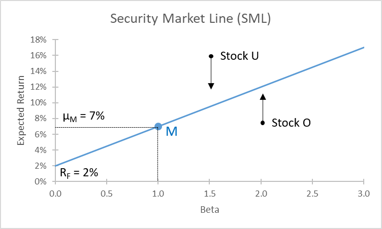
The graphical representation if the Capital Asset Pricing Model is the so-called Security Market Line (SML), which shows the expected return of efficiently priced assets as a function of the beta of these portfolios:
In equilibrium, and under the assumptions made above, all individual assets should lie on the security market line (SML): Their expected rate of return should correspond to the risk free rate (\(R_F\)) plus a compensation for their systematic risk. This compensation equals the beta of the asset (horizontal axis) times the market risk premium.
- An asset that lies above the SML (Stock U in the graph above) offers a higher expected return than could be justified by the CAPM. Therefore, its current price is too low, according to the CAPM—it is undervalued. This will attract investors who buy the asset. As a result of the buying, the price goes up and the expected return comes down. Investors will buy until the asset is fairly priced, given its systematic risk. The undervaluation is cured when the asset is (back) on the SML.
- Similarly, an asset that lies below the SML (Asset O in the graph above) offers a return that is lower than its CAPM return. Consequently, the asset is overpriced. Investors will sell it and thereby push the price down and the expected return up. Selling will stop when the asset is (back) on the SML.
After all the theoretical considerations, let us practice this relation with a few examples.

