Reading: Estimating the Cost of Capital
4. Beta
The last element of the CAPM-equation is the beta of the project, \(\beta_j\). As we have seen in the theoretical considerations, beta captures the systematic risk of the asset in question:
\( \beta_j = \frac{\sigma_j \times \rho_{Mj}}{\sigma_M} \)
To estimate the beta of an asset, we therefore need to have information about its volatility (\(\sigma_j\)), the correlation with the market return (\(\rho_{Mj}\)) and the the riskiness of the market (\(\sigma_M\)). If we have historical returns, we can estimate these parameters just the way we did in the section on the distribution of returns.
Technically speaking, we obtain the same when estimating the following regression equation:
\( r_{j,t} = \alpha_j + \beta_j \times r_{M,t} + \epsilon_{j,t} \),
where \(r_{j,t}\) is the continuously compounded return on the asset; \(r_{M,t}\) is the continuously compounded return on the market portfolio; \(\alpha_j\) is the intercept; \(\beta_j\) is the slope of the regression line, and \(\epsilon_{j,T}\) is the error term.
Graphically speaking, such a regression plots the returns of the asset and the market portfolio in a two-dimensional space and then fits a line through the data points that explains the returns as well as possible. The slope of that line is the beta coefficient that we are looking for.
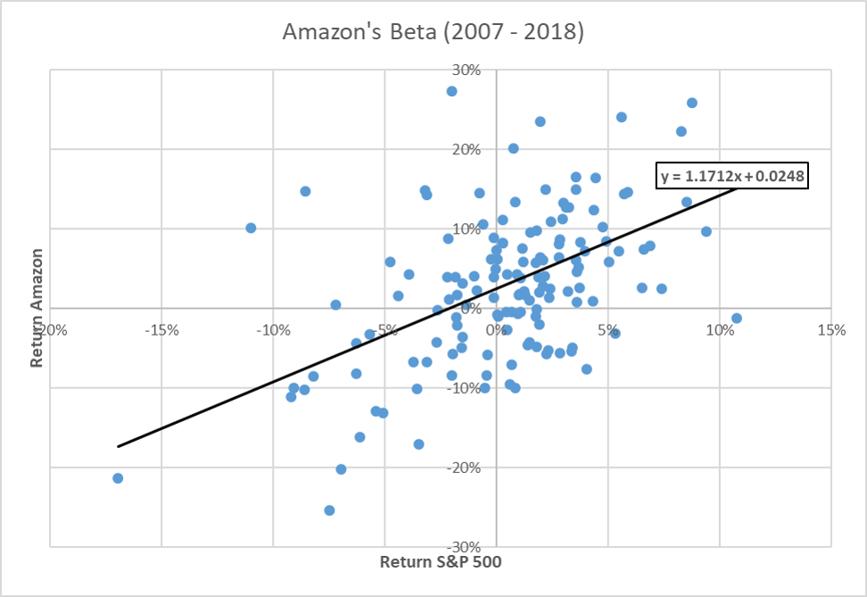
As an illustration, the following graph shows the result of this procedure for Amazon:
- Each data point describes the return on Amazon's stock (vertical axis) and the return on the market portfolio (approximated with the S&P500 stock index) in any given month between January 2007 and January 2019.
- The solid black line is the straight line that best explains these data points.
- The slope of that line is 1.17. That's Amazon's beta based on monthly returns against the S&P500 index over the period 2007-2019.
As mentioned above, we obtain the same result when estimating the volatilities and the correlation separately and plugging the values in the beta-equation. In this particular case, we have: \(\sigma_{text{Amazon}}=0.1019\); \(\sigma_{\text{SP500}}=0.0424\); \(\rho_{\text{Amazon,SP500}} = 0.4869\). Consequently:
\( \beta_{\text{Amazon}} = \frac{\sigma_{\text{Amazon}}\times \rho_{\text{Amazon,SP500}}}{\sigma_{\text{SP500}}} = \frac{0.1019 \times 0.4869}{0.0424} = 1.17 \)
Not surprisingly, there is also a pre-built Excel function that allows us to compute the lope coefficient of a regression. The command is "=SLOPE()".
A simple practical approach
Admittedly, the above procedure is too cumbersome for most applications. Therefore, a good first-pass approximation is to refer to one of the many online sources that provide information about beta coefficients. In the particular case of Amazon, we have:
| Source | Amazon's Beta |
| Yahoo Finance | 1.71 |
| Marketwatch | 1.34 |
| Reuters | 1.68 |
| Nasdaq | 1.42 |
As we can see, different sources provide quite different values. Most likely, the reason is that they consider different data frequencies and periods. In the regression above, we have used monthly data over 12 years. Other sources might use monthly data over 3 years or 5 years and yet other sources might rely on weekly or daily data.
This illustrates a very important point. Estimating these parameters is not an exact science. We have to understand that our estimates are most likely affected by measurement error and we have to make sure that we know ow to cope with measurement error. One way to do so would be to estimate the cost of capital with different betas and then investigate whether the NPV of the project remains positive in the various scenarios. The section "Coping with Measurement Error" of the module Firm Valuation takes a closer look at this important issue.