Reading: Portfolio with Multiple Assets

This section presents the relevant formulas for calculating the return and risk of portfolios with more than two risky assets. Naturally, this section is rather technical. The fundamentals conveyed herein are NOT central for further understanding diversification and estimating the cost of capital. Therefore, the hurried reader can safely skip this section...

When transitioning from portfolios with two risky assets to a world with N risky assets, the return and risk of the portfolio are determined by the following equations:

Expected return of Portfolio P: \( \mu_P =\sum_{i=1}^{N}w_i\mu_i \)

Variance of Portfolio P's return: \(\sigma_P^2=\sum_{i=1}^{N}w_i^2\sigma_i^2+\sum_{i=1}^{N}\sum_{j=1}^{N}w_{i}w_{j}\sigma_{i}\sigma_{j}\rho_{ij}\)

Standard deviation of Portfolio P's return: \( \sigma_P = \sqrt{\sigma_P^2} \)

These formulas suggest that calculations for portfolios with many assets quickly become complex. Therefore, implementing them in Excel is recommended, as we'll demonstrate below.

Application Example: Portfolio with 5 Assets

Let's consider a portfolio composed of 5 assets (A, B, C, D, and E) (see accompanying Excel file):

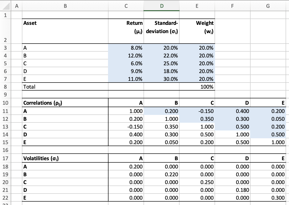
• In column C, the following image displays the expected returns (\(\mu_i\)) and in column D, the standard deviations of these returns (\(\sigma_i\)) for the 5 assets.
• The correlations of the individual assets (\(\rho_{ij}\)) are also depicted. The respective values are within the correlation matrix spanning from C11 to G15. Note that the diagonal always assumes a value of 1, as an asset perfectly correlates with itself. Furthermore, the values above the diagonal mirror those below it, for example, the correlation between Asset A and B (cell D11) must be the same as between Asset B and A (cell C12).
• It also presents the individual standard deviations (from column D) in tabular form. This representation will help us keep the calculations "simpler" later on.

Now, let's assume we want to construct a portfolio that equally invests in the 50 assets, assigning each of them a weight of 20% (w_i). This is known as the "1/N-Portfolio," which enjoys a certain popularity in practice. 

Expected Portfolio Return (\(\mu_P\))

To calculate the expected portfolio return, we multiply each asset's weight in the portfolio (w_i) by its expected return (\(\mu_i\)) and sum up the resulting values. Technically, this can be implemented in Excel using the "SUMPRODUCT" function:

Expected Portfolio Return (\(\mu_P\)) = SUMPRODUCT(C3:C7;E3:E7) = 9.20%

Standard Deviation of Portfolio Return (\(\sigma_P\))

As the formula above suggests, calculating the portfolio's risk appears somewhat cumbersome. The portfolio variance results from the combination of weights with variances and covariances, and can be derived through a series of matrix multiplications in Excel:

Portfolio Variance (\(\sigma_P^2\)) = =MMULT(MMULT(MMULT(MMULT(MTRANS(W);V);C);V);W)

where:

• W: a 1xN vector describing the portfolio weights (E3:E7)
• V: an NxN matrix with the individual volatilities (C18:G22)
• C: an NxN correlation matrix (C11:C15)
• MMULT() is a function in Excel for multiplying two matrices
• MTRANS() is a function in Excel for transposing a vector

When entering the respective values in Excel, we find a portfolio variance of 0.021:
 

\(\sigma_P^2\) = MMULT(MMULT(MMULT(MMULT(MTRANS(E3:E7);C18:G22);C11:G15);C18:G22);E3:E7) = 0.021

Calculating the standard deviation of the portfolio return is relatively simple now; it results from the square root of the variance:
 

\(\sigma_P = \sqrt{\sigma_P^2} = \sqrt{0.021} = 0.1451 = 14.51\%\)

Under the given assumptions, a portfolio that invests 20% of the wealth in assets A, B, C, D, and E has an expected return of 9.2%, with a standard deviation of 14.51%. These calculations are summarized in cells C25 (portfolio return) and C29 (standard deviation) of the attached Excel file.

The following graph illustrates the 5 assets along with the just calculated 1/N-Portfolio in the familiar risk-return space:

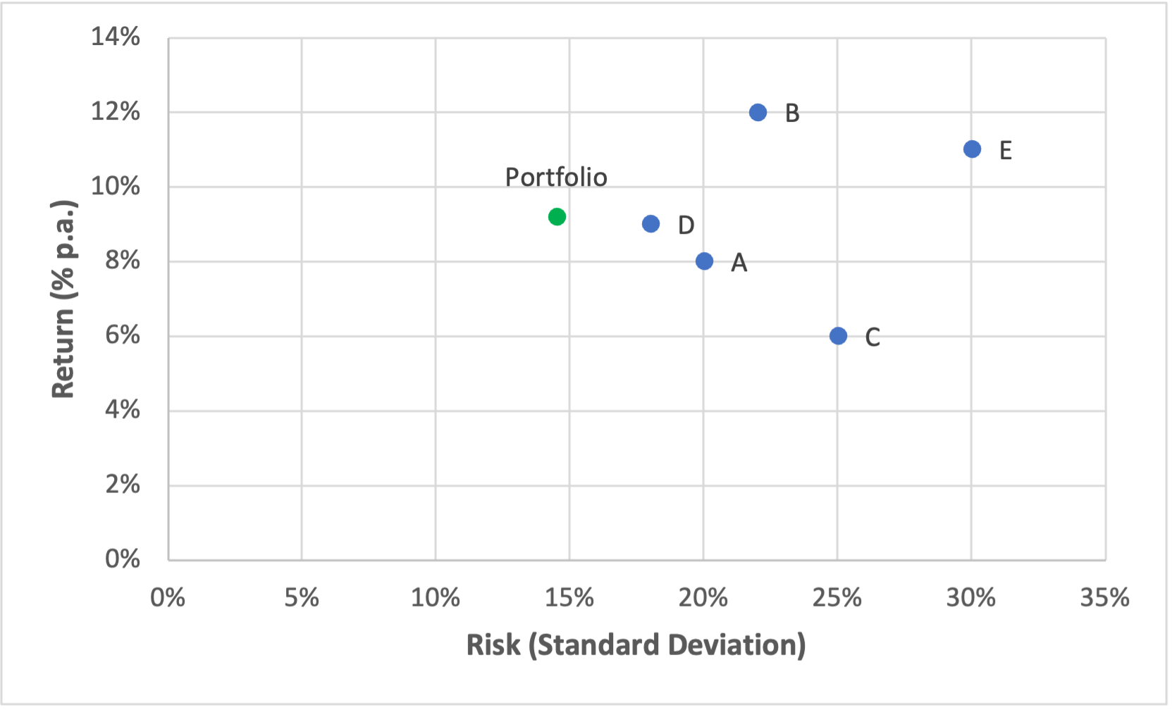
Again, we see the benefit of diversification: Our portfolio achieves a higher return than assets A, C, and D while simultaneously exhibiting significantly lower risk. 

Portfolio Optimization

By choosing different portfolio weights (cells E3 to E7), we can now calculate any desired portfolios. For instance, we could search for the portfolio with the lowest risk, known as the Minimum Variance Portfolio. 

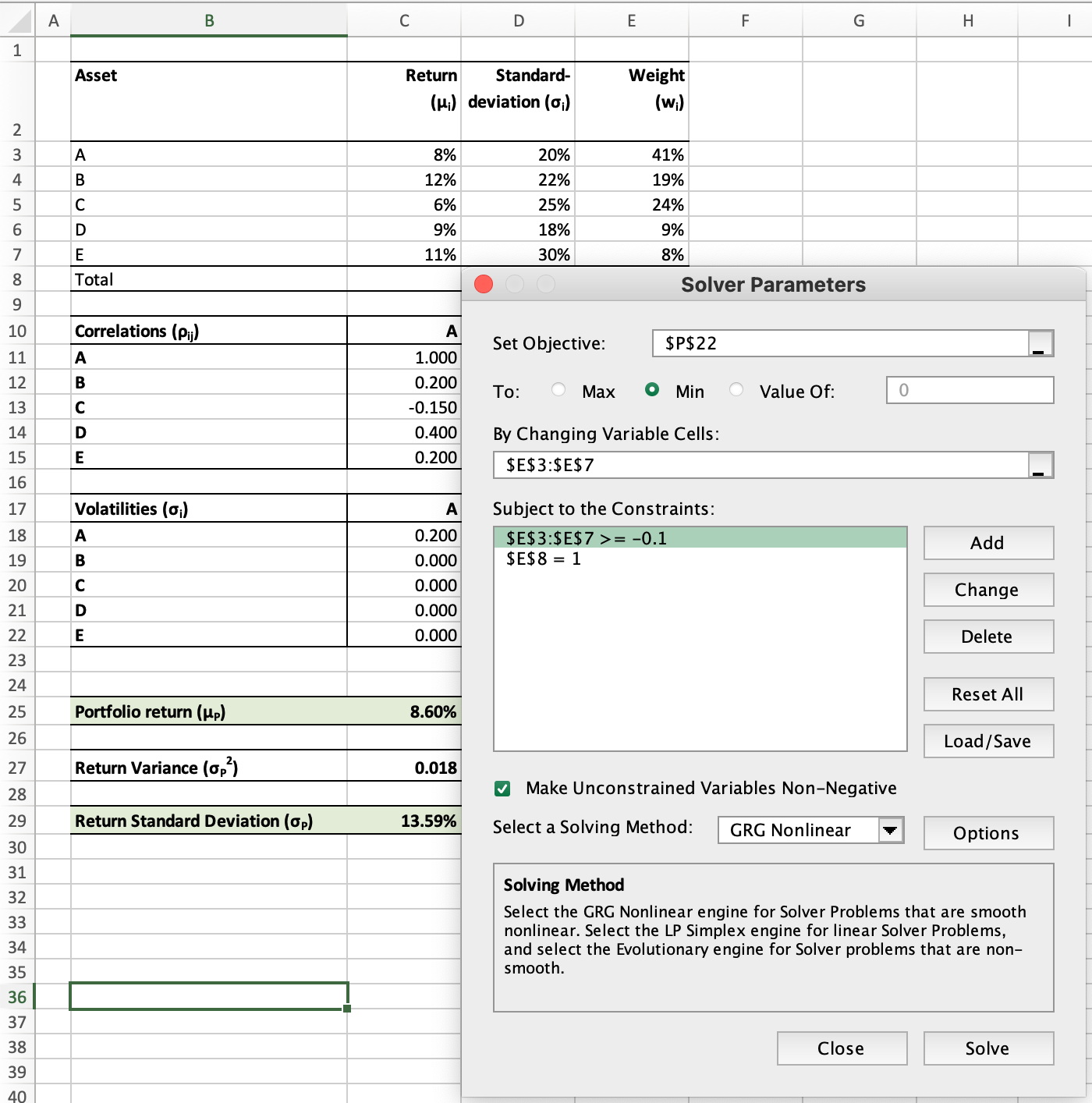
This can be easily accomplished in Excel using the "Solver" add-in. With this add-in, simple optimizations can be directly implemented in Excel. In the present case, we would instruct the Solver as follows (see Sheet "MVP" in the Excel File):

In words:

• The objective is to minimize the standard deviation of the portfolio return. Thus, we instruct the Solver under "Set Objective":
  • C29 (the cell with the portfolio return)
  • Min. (Minimize)
     
• The Solver can find different portfolios by working with different portfolio weights (w_i). Accordingly, we instruct:
  • "By changing cells:" E3:E7 
     
• During optimization, the Solver must satisfy some constraints. For example:
  • 100% of the capital must be invested (otherwise, all portfolio weights would be set to 0, resulting in a risk of 0). 
  • To achieve this, we add a constraint demanding that the sum of portfolio weights (in cell E8) equals exactly 1.
  • Finally, we can determine whether there are certain upper or lower limits for each asset. In the presented optimization, for instance, it was assumed that no asset can have a weight of less than -10% (a so-called "short position").
     
• Once the Solver is fully calibrated, the optimization can be initiated by clicking "Solve."
  • The resulting portfolio invests 41% in Asset A, 19% in B, 24% in C, 9% in D, and 8% in E (see image above). 
  • This Minimum Variance Portfolio (MVP) has a return of 8.6% with a standard deviation of 13.69%.

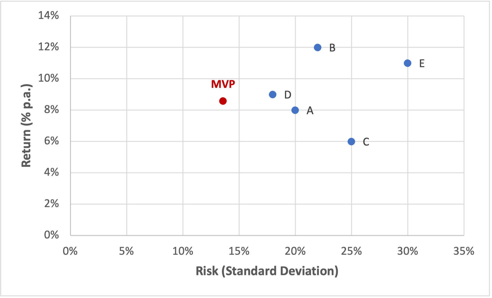
The Minimum Variance Portfolio is plotted in red in the graph below. Compared to the 1/N-Portfolio, it exhibits slightly lower risk (with a correspondingly lower return). Following the same logic, we could use the Solver to compute the Efficient Frontier.

This section has provided the necessary technical tools to evaluate portfolios with more than two assets in terms of risk and return.